As the cost of DNA sequencing and downstream data processing continues to decrease, population sequencing studies are becoming feasible at unprecedented scales. Cohort-level catalogs of variation are key resources for ancestry studies, rare variant analysis, and genotype/phenotype associations discovery. It is therefore important that call sets are highly accurate, yet data processing and analysis challenges remain.
Several tools exist to aggregate call sets from large cohorts. One example is GATK and its Joint Genotyping workflow,1 which has set the standard for many years. However, it contains several steps that are only required for variant sets called by GATK and do not apply to other variant callers, such as variant score recalibration (VQSR). There is also GLnexus,2 developed by DNAnexus and tightly coupled to their cloud platform. It is not obvious how to deploy it at scale on other cloud platforms or on HPC. Another challenge for many existing tools is an efficient iterative analysis, allowing the addition of new samples and their variants to an existing call set.
DRAGEN gVCF Genotyper is Illumina's solution to aggregate and genotype small germline variants at population scale. The input to gVCF Genotyper is a set of gVCF files3 written by the DRAGEN germline variant caller. The output is a multi-sample VCF file (msVCF) with genotypes for all variants discovered in the cohort. The output will also contain cohort metrics that can be used for quality control and variant filtering.
DRAGEN gVCF Genotyper implements an iterative workflow to add new samples to an existing cohort. This workflow allows users to efficiently combine new batches of samples with existing batches without repeated processing.
Users can ingest the output msVCF into downstream tools, like Hail (https://hail.is) and PLINK (https://www.cog-genomics.org/plink), for data exploration or to perform association studies.
In this article, we give an overview of the gVCF Genotyper workflow, show how to deploy it at scale, and demonstrate the performance of the DRAGEN gVCF Genotyper using the 1000 Genomes Project (1KGP) cohort.
We have used gVCF Genotyper in several internal projects, for instance a reanalysis of the 1KGP cohort (https://www.internationalgenome.org) using DRAGEN 4.0 and larger cohorts with up to 500,000 samples. External users include Genomics England4,5 and others.
The software is part of DRAGEN, Illumina's solution for the analysis of next-generation sequencing data. In DRAGEN 4.0, gVCF Genotyper can scale to hundreds of thousands of samples when using the distributed processing mode. Our recommended—and the most scalable—platform on which to execute gVCF Genotyper is Illumina Connected Analytics (ICA), but we also support on-premise analysis on DRAGEN servers and HPC deployment.
Genotyping at scale
DRAGEN gVCF Genotyper relies on the gVCF input format, which contains both variant information, like a VCF, and a measure of confidence of a variant not existing at a given position (homozygous reference positions).
The genotyping workflow consists of several steps: First, we extract the variant alleles from each input file. We store the variant genotypes and other metrics. In the next step, we collect variant sites that capture all alleles at a position. We apply filters and discard alleles with low quality and alleles not supported by a called genotype. This includes using information from samples that are homozygous reference at this position.
After this, the variant alleles are normalized. We compute an allele map from the index of an allele in the input to the allele order in the site. An example is given below (Table 1). We also update the genotypes and QC metrics from each sample to match the normalized set of alleles.

A scalable VCF representation
The output of gVCF Genotyper is an msVCF that contains metrics computed for all samples in the cohort.
With increasing cohort size, the msVCF can become large—in some cases requiring more memory than can be allocated by VCF parsers, causing challenges to memory and run time. This is caused by VCF entries that store values for each possible combination of alleles, such as FORMAT/PL, and therefore scale quadratically with the number of alleles. In low-complexity regions of the genome, the number of alleles per site can be large. It will also increase drastically with the number of samples.
For all these reasons, we replaced FORMAT/PL with the tag FORMAT/LPL, which stores a value only for the alleles occurring in the sample and not all alleles found at this site in the cohort. We also added a new FORMAT/LAA field for each sample, which lists 1-based indices of the alternate alleles that occur in this sample with respect to the global list of alleles.
This approach is referred to as local alleles and is also used by open-source software such as BCFtools (https://samtools.github.io/bcftools/bcftools.html) and Hail (https://hail.is/docs/0.2/experimental/vcf_combiner.html#local-alleles).
The msVCF also contains allele counts for each allele and the inbreeding coefficient. Allele counts are used to compute allele frequencies, which, among other things, are a useful metric to decide whether a variant is likely benign or might be pathogenic.
The inbreeding coefficient (IC) measures the excess heterozygosity at a variant site. It can also be used to detect and filter read mapping artifacts:6 positions in the genome with high excess heterozygosity can be regions with incorrect read mappings that appear heterozygous because some reads in fact belong to a different part of the genome.
We calculate the inbreeding coefficient as 1 − (number of observed heterozygous genotypes) / (number of expected heterozygous genotypes). If this quantity is negative, it means that we have observed more heterozygotes than expected given Hardy-Weinberg assumptions (https://en.wikipedia.org/wiki/Hardy%E2%80%93Weinberg_principle).

A good rule of thumb is to filter variant sites with a negative inbreeding coefficient.6 Figure 1 illustrates why this is a useful approach: A negative inbreeding coefficient captures sites with a high heterozygosity that are not filtered by other filters, such as call rate (NS_GT).
Below is an illustration of an msVCF file that was written by DRAGEN gVCF Genotyper and that uses the “local alleles” formalism as explained (Figure 2).

Open-source software like GATK is writing the full set of genotype likelihoods (FORMAT/PL), whereas DRAGEN gVCF Genotyper and other tools such as Hail write a reduced set for only the alleles that actually occur in the sample (“local alleles”).
Comparison to GATK best practices
The GATK (Genome Analysis Toolkit) best practices recommend several steps to analyze variant calls from a large cohort, including recalibration of quality scores, ingestion into a database, and a refinement of genotypes (also referred to as joint genotyping).
Joint genotyping refers to a class of algorithms that leverage cohort information to improve genotyping accuracy. The GATK team was the pioneer of this methodology.
Improving genotyping accuracy is important, but we have shown7 that a GATK-style algorithm for joint genotyping is not required for DRAGEN variant calls, as it does not lead to a gain in accuracy. The reason is that the GATK algorithm tries to remove variant artifacts, however these have already been filtered upstream in DRAGEN.
Since the GATK joint genotyping algorithm is also a computationally expensive operation, we recommend users run only DRAGEN gVCF Genotyper without GATK-style joint genotyping on DRAGEN variant calls.
The same applies to VQSR, which is no longer recommended for variant call sets using recent versions of DRAGEN (https://community.illumina.com/s/question/0D53l00006lvBDBCA2/why-vqsr-was-removed-from-latest-versions-of-dragen).
Single server analysis versus distributed processing
The gVCF Genotyper workflow can be run in a step-by-step mode if multiple batches of samples are available, or single server analysis mode if only a single batch of samples is available.
The FASTA reference used for gVCF Genotyper must be the same as that used to build the DRAGEN hash table for alignment and variant calling.
The single server analysis mode takes a set of gVCF input files and aggregates them into a single msVCF. It is useful to quickly generate an msVCF with metrics and genotypes for a limited number of samples. In this mode, iterative analysis is not possible.
Details of the single server analysis workflow are given in the DRAGEN 4.0 user guide.8

The step-by-step mode as depicted in Figure 3 consists of several steps to distribute the compute across several nodes. The workflow scales to several hundreds of thousands of samples.
Step 1 (gVCF aggregation): Aggregate a batch of gVCF files into a cohort file and a census file. The cohort file is a condensed data format to store gVCF data from multiple samples, similar to a multi-sample gVCF. The census file stores summary statistics of all variants and blocks of homozygous reference genotypes for each sample in the cohort. When many samples are being processed, the user should divide them into multiple batches each of a similar size (for example, 1000 samples), and run Step 1 on every batch separately.
Step 2 (census aggregation): After all batch census files are generated, the user can merge them into a single global census file. This step scales to thousands of batches.
Step 3 (msVCF generation): Once the global census file has been generated, the user can use it with the per-batch cohort and census files, to generate msVCF files for each batch of samples.
To facilitate parallel processing on several compute nodes, for every step above, the user can choose to split the genome into shards of equal size (using the command line option –shard described in the user guide) and process each shard using one instance of iterative gVCF Genotyper on a different compute node. Genomic shards are broken at chromosome boundaries, imposing a lower bound on the number of shards.
This workflow results in (number of sample batches) * (number of genomic shards) msVCF output files. If a combined msVCF of all batches is required, an additional step can be run to merge all the batch msVCF files into a single msVCF containing all samples.
When a new batch of samples becomes available, the user needs only to perform Step 1 on that batch, then combine the census file from the new batch with the global census file from all previous batches and write a new global census file. Every time a global census file is updated, with new variant sites discovered and/or variant statistics updated at existing variant sites, new batch-wise msVCF files can be generated that contain the new information.
Below, Figure 4 shows the steps that are required to add a new batch of samples to an existing cohort. For the gVCF files in the new batch, only Step 1 must be executed to build a new per-batch cohort and census file. After this, the workflow will execute Step 2 to build the new global census file that is needed to update the msVCF files for each batch in Step 3.

Availability in the cloud and on premise
DRAGEN gVCF Genotyper is part of DRAGEN 4.0 and can run on a DRAGEN server, like all other components. However, this is feasible only for small cohorts: 1000 gVCF files will take about 24 hours in single server analysis mode.
A workflow to run the iterative gVCF Genotyper is implemented in ICA and is our recommended option for users with large cohorts (> 10,000 samples). The ICA workflow has been tested with more than 100,000 germline samples.
gVCF Genotyper is available on the ICA platform. For ICA v2, a command line interface (CLI) is available.11
The cost of running gVCF Genotyper in ICA is approximately 0.3 iCredits/sample for single server analysis workflow from gVCF to msVCF. The cost for an iterative analysis is approximately 0.3 iCredits per new sample added and 0.06 iCredits to update the msVCF for each already processed sample. This estimate is based on DRAGEN 4.0 running on 500 cores and ICA running in the AWS region us-east-1.
In most cases, the platform allows users to trade off costs versus run time—for instance, using fewer ICA nodes will cost less, but will increase the time to result.
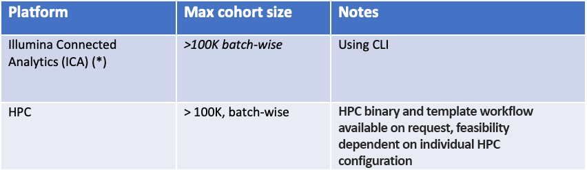
We also offer a software-mode binary of gVCF Genotyper that can be run on commodity hardware and on an HPC.
The run time of gVCF Genotyper is dependent on the speed of disk I/O. The size of the input files is also an important factor.
When planning for a gVCF genotyping project, consider therefore using the compact gVCF output mode in the DRAGEN germline variant caller (command line option --vc-compact-gvcf). This results in gVCF files that are 40%–50% smaller and can give a significant speed-up in software that parses the files, such as gVCF Genotyper. Storage costs are also reduced. This compact gVCF mode omits some metrics from the gVCF that are needed only for the de novo detection of variants in pedigrees, meaning that the compact gVCF cannot be used with the DRAGEN pedigree caller.
Use case: Analysis of The 1000 Genomes Project in ICA
Seven years ago, 1KGP published an open-access data set consisting of low-coverage sequencing (data of 2504 unrelated individuals from 26 populations). This was the first large-scale sequencing effort to compile a catalog of human genetic variation.
Researchers at the New York Genome Center, in collaboration with other scientific partners, have expanded this resource to include many parent-child trios. The expanded set consists of 3202 samples, including 602 trios, and is publicly available.9
The New York Genome Center used GATK to call variants in this cohort. Illumina has reanalyzed the samples using DRAGEN 4.0 and made it publicly available. This data release will be described in a separate blog post.
We used DRAGEN gVCF Genotyper to aggregate and genotype all 3202 samples. The cost for the analysis was 990 iCredits, equivalent to 0.31 iCredits per sample. The result of this analysis is an msVCF containing genotypes and frequencies for all variants in the cohort. We also collected statistics on missing genotypes and deviations from Hardy-Weinberg assumption as expressed by the inbreeding coefficient (Figure 1).
We demonstrate the versatility and accuracy of the genotyped msVCF using two examples:
Mendelian inconsistent genotypes in a hidden trio
We computed Mendelian error rates in a hidden trio that was part of the cohort10—samples NA20891, NA20882, NA20900. Counting genotype calls that violate family relationships is a useful metric for assessing accuracy because they are not limited to the high-confidence regions of the genome.
Below, Table 3 shows the number of Mendelian errors over the total number of sites for which at least one member of the trio has a variant. The table compares the GATK call set to call sets generated with DRAGEN 4.0 and 3.5.7.

Analysis of putative cell line artifacts in 1KGP
The New York Genome Center did an analysis of variants that occur only once in the whole cohort (singletons, allele count [AC]=1).9 Their hypothesis was that many of these variants are artifacts of the cell lines. They also compared the number of singletons in samples with relatives in the cohort to their number in samples without relatives. Children have the lowest number of singletons, followed by parents and then samples without any relatives in the cohort.

DRAGEN gVCF Genotyper computes many variant metrics on the fly, among them allele counts. Therefore, singleton variants can readily be extracted and analyzed without resorting to other tools. Above, Figure 5 shows a breakdown of singleton variants per sample. The plot shows how samples segregate according to their relatedness status; children tend to have the fewest singletons, followed by parents and unrelated samples.
For more information or a DRAGEN trial license for academic use, please contact dragen-info@illumina.com.
References
1. Derek Caetano-Anolles (2022) “Calling variants on cohorts of samples using the HaplotypeCaller in GVCF mode” https://gatk.broadinstitute.org/hc/en-us/articles/360035890411-Calling-variants-on-cohorts-of-samples-using-the-HaplotypeCaller-in-GVCF-mode
2. Michsel F Lin (2018) “GLnexus: joint variant calling for large cohort sequencing “ https://www.biorxiv.org/content/10.1101/343970v1
3. Derek Caetano-Anolles (2022) gVCF – Genomic Variant Call Format https://gatk.broadinstitute.org/hc/en-us/articles/360035531812-GVCF-Genomic-Variant-Call-Format
4. Kousathanas et al (2022) “Whole-genome sequencing reveals host factors underlying critical COVID-19” https://www.nature.com/articles/s41586-022-04576-6 Nature volume 607, pages 97–103
5. Genomics England press release on covid 19 patient study https://www.genomicsengland.co.uk/news/study-insights-severe-covid-19
6. Derek Caetano-Anolles (2022) “Inbreeding coefficient” https://gatk.broadinstitute.org/hc/en-us/articles/360035531992-Inbreeding-Coefficient
7. Population genetics data processing with the DRAGENTM Bio-IT Platform https://jp.support.illumina.com/content/dam/illumina/gcs/assembled-assets/marketing-literature/dragen-popgen-tech-note-m-gl-00561/dragen-popgen-tech-note-m-gl-00561.pdf
8. Instructions for using the Illumina DRAGEN Bio-IT Platform https://support-docs.illumina.com/SW/DRAGEN_v40/Content/SW/DRAGEN/gVCFGenotyper.htm
9. Marta Byrska-Bishop et al (2022) “High-coverage whole-genome sequencing of the expanded 1000 Genomes Project cohort including 602 trios” Cell, Volume 185, https://www.cell.com/cell/fulltext/S0092-8674(22)00991-6#%20
10. Roslin N, Li W, Paterson AD, Strug LJ. Quality control analysis of the 1000 Genomes Project Omni2.5 genotypes. bioRxiv. 2016;078600–078600.
11. The PopGen CLI is available as a bundle in ICA. Its name depends on their ICA subscription region. We currently have entitled bundles in the following 3 regions:
a. US East (use1) entitled bundle name "popgen-cli-release-use1"
b. London (euw2) entitled bundle name "popgen-cli-release-euw2"
c. Singapore (apse1) entitled bundle name "popgen-cli-release-apse1"